Guided Introduction to iolite Targeting

Below you will find short guides to using iolite Targeting (hereafter “Targeting”). The first guide introduces the concept of ‘Regions’ in Targeting. This is followed by the first practical example which is a basic grain finding example on a simple image. You can follow along with this example by downloading the example image file. While this first example is the longest, it introduces most of the concepts that you will use regularly in Targeting regardless of the application such as setting up the experiment run order and adding reference material patterns.

The second practical example demonstrates how to create lasso patterns for imaging experiments and uses a TIFF image from an SEM that contains embedded coordinate information. The third example shows how to import a point analysis file (e.g. SEM point analyses) and use these for creating ablation spot patterns at the same location. It also shows how to include the compositional information as metadata for later use in iolite or storage in a database. The fourth example shows how to load an image from an existing iolite experiment (.io4) file. The fifth example demonstrates how to use Targeting’s advanced segmentation training features to segment an image into separate phases. And finally, the seventh example demonstrates how to use Precognition to find the optimal conditions for your imaging experiments.

Introduction: Regions

Targeting is based on :term:Regions. A region typically represents a grain mount or thin-section, and you will typically have several regions in an experiment. A key feature of a region is that after re-coordination, the relative distances and angles between lines in the region remain the same, even with some amount of rotation and scaling applied. An example showing this is shown in Fig. 8. Note that multiple grain mounts would not be processed as a single region as after loading in the cell, each grain mount might be rotated by a slightly different amount, which would violate the principle of conserved angles and relative distances.

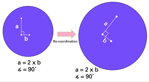
Fig. 8 A diagram showing an example region representing a grain mount with three points for ablation. After re-coordination, the relationship between distances and angles remains the same for the region.

Regions can contain any of the following: images, data points (e.g. from an SEM point analysis file), alignment points, and ablation patterns.

Regions are shown in the top left of the Main Window, and are in a tree structure. Clicking to expand a region will show subfolders for the alignment points, images, data, and ablation patterns of that region. Clicking on any one of these subfolders will show the component images etc. Clicking on an item will show its properties in the Properties Panel, which is in the bottom left by default.

Clicking on an ablation pattern (e.g. spot, raster etc) will show the ablation properties of that pattern, including spot size, rep rate, fluence etc in the Properties Panel. The properties shown will depend on the pattern type.

Example 1: Basic grain finding

You can use this example image (NOTE: this image is around 60 MB) to practice the basic concepts introduced below. However, to follow the full process you will need a physical grain mount and accompanying image to load it into the cell and complete the re-coordination process.

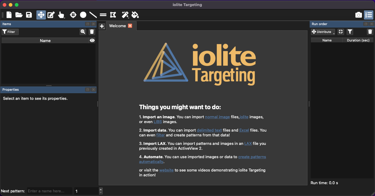
Fig. 9 A screenshot showing the welcome tab of iolite Targeting

Start a new Targeting session. When a new Targeting session starts, the Welcome tab (shown in Fig. 9) is visible. An overview of the user interface is available in the Main iolite Targeting Window.

Importing an Image

New regions can be created by clicking the button (to the left of the Welcome tab; highlighted in orange in Fig. 10.

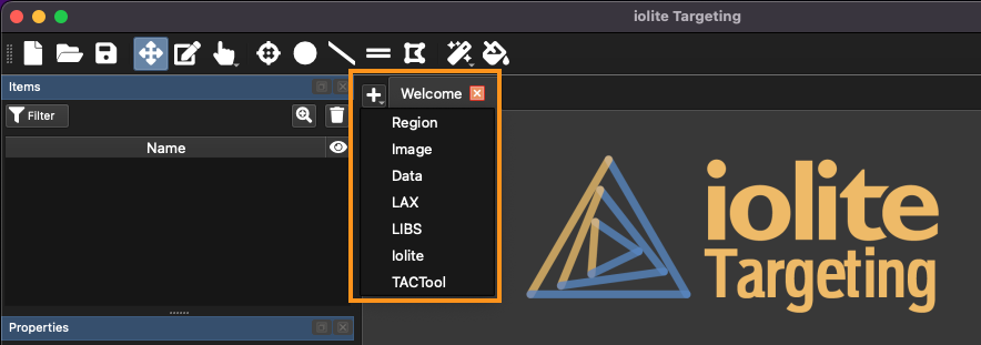
Fig. 10 A screenshot showing the location of the import button menu

Using this menu, you can import images, data files, iolite experiments, raw LIBS files, existing LAX files (from AV2) and create blank regions. In this case, we’ll import a new image. Click Image from the menu and select your grain mount image (or the example image). The Import Image window will open, and Targeting will process the image. This includes ensuring that the image zooms in and out smoothly. The size of the image will determine how long the image processing takes (usually <15 seconds for a large image). At the top of the Image Import window are two options: import type, and scale.

The first option is whether to import the image as a new region, or to add to an existing region. In this example we will create a new region, so this option can be left as is. The second option is how to define the scale of the image. Depending on the option chosen, the user can input the Width or Height dimension (in micrometers) or if a scale bar is present on the image, the Scale Bar option can be selected. If the latter is selected, the user can left click and drag a line over the scale bar, and then after clicking OK, the length of the scale bar can be entered. A later example will use this method.

If the image contains metadata about the scale and position of the image, such as some SEM images, another option will be available in the Scale dropdown menu: Embedded Information. Using this option avoids having to set the image position and scale. If the image does not contain the relevant metadata, this option will not be present.

Click OK to import the image and define the scaling. If using the example image, the image width is 25000 micrometers.

Note

If an incorrect scaling value is entered in Targeting, it will be corrected during the re-coordination process in the laser control software. However, it will affect stats calculated by Targeting such as the grain area etc.

A new region will then be shown in the Regions list (top left of window, Fig. 11). At this point, the region only contains a single image.

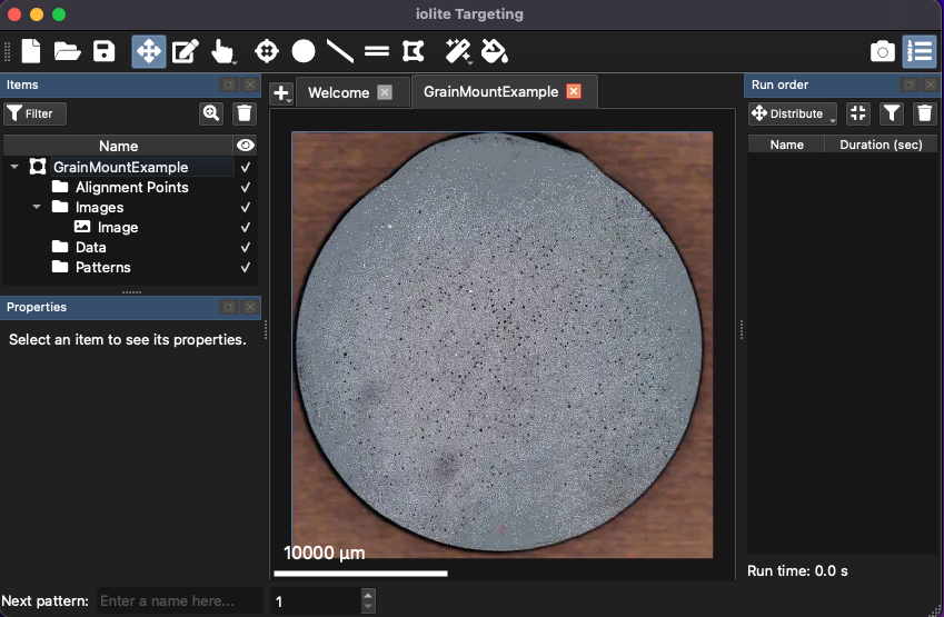
Fig. 11 A screenshot showing an imported image and corresponding region

Tip

You can zoom in and out in Targeting by holding the Ctrl key (Cmd key on Mac) and scrolling the mouse wheel.

Threshold Targeting

To place a spot on each grain, begin the grain finding process by clicking the button. Click and hold this button to show automatic detection options.

Note

Buttons in Targeting with a small down arrow in the bottom right have additional options that can be accessed by clicking and holding the button. The button is an example of a button with additional options accessed in this way.

There should be two options: threshold (using a threshold value to find grains) and training (using defined regions to find similar regions). Ensure threshold is selected, and then click the button again to make it active (it will be highlighted when active).

When the button is active, you can draw a area in the image to identify grains in. This can be the entire image, or a subset of the image if there are extraneous features in the image. Use the mouse to left click and drag out an area for grain detection, starting in the top left of the intended area and then the bottom right of the area.

Tip

If using the example image, there are ablation pits on grains in the lower right quadrant of the mount. You may want to avoid these to make the example simpler. There are many thousands of grains in the example image. Selecting only around 15% of the image should be sufficient for the example.

Once the area for grain identification is selected, the Threshold Targeting window will appear (Fig. 12). There are three tabs across the top of this window: Source, Find and Target. The source tab shows the source image (i.e. the image used in the grain detection algorithm). The Find tab shows options for detecting the grains, and the Target tab shows options for placing ablation patterns.

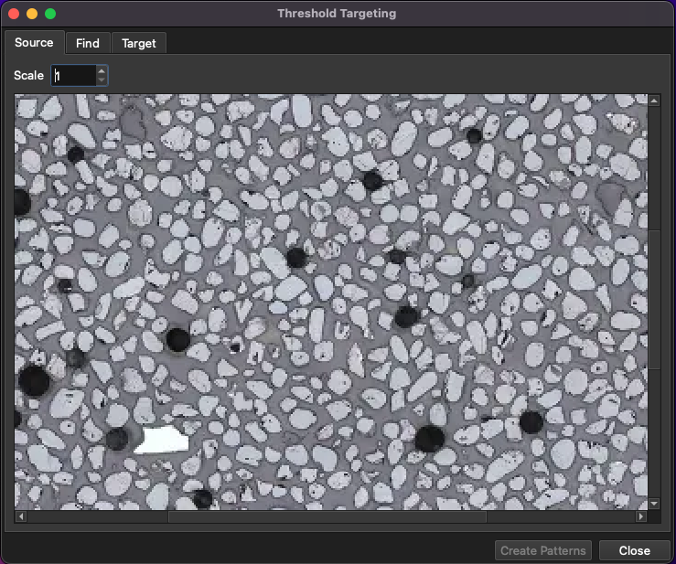
Fig. 12 A screenshot of the Threshold Targeting window

The Find tab will show the selected region, which can be zoomed in and out by holding the Ctrl key (Cmd key on Mac) and scrolling the mouse wheel. This tab helps check the correct area has been selected. The scale control at the top of the Find tab can be used to scale down the image of the selected area. It is not required in this example.

In the Find tab, there are settings for the grain detection algorithm. In short, grains are detected by creating a thresholded image where pixels in a user-defined range are all set to 1 and all other pixels are set to 0. The algorithm then creates contours around the areas set to 1. These contours represent the grain boundaries. To set the areas to be defined as grains, set the pixel values associated with the grains by clicking the Histogram button. This will show a histogram of pixel values within the selected area (Fig. 13). By default this will show the pixel values converted to grey-scale. In the bottom left, there are options for showing the red, green and blue pixel values (only for color images). There are two dashed lines on the histogram representing the upper and lower thresholds. Pixels between these thresholds will be set to one in the thresholding process of the algorithm. You can click and drag these thresholds to select the pixels representing your grains.

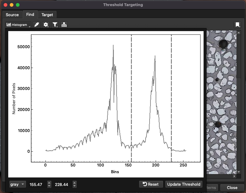
Fig. 13 A screenshot showing the histogram used for setting thresholds in grain detection

If using the example image, the zircon grains are mid to light grey colors, so you can use the thresholds shown in Fig. 13. If your image was a color image and all the grains of interest were colored red by some other program, you could show the red pixel histogram using the control at the bottom right and selecting the high red intensity and low green and blue intensities to select your grains.

Once you have selected your pixel value thresholds, click the Update Thesholds button at the bottom right of the Histogram window. The grain finding algorithm will work in the background and identify grains. Click the Histogram button again to hide the Histogram window.

An alternate way to select the pixel value ranges is to click the button and then click on the grains of interest. For reasons of succinctness, this is not covered here.

Each grain detected by the algorithm will be outlined by a colored boundary. Settings for refining the algorithm are available in the , and buttons.

In the button options there are settings for “smoothing” and “opening”. Smoothing will apply a Gaussian or blur filter to the selected area image and the setting shown in this menu refers to the size of the smoothing kernel: larger kernels smooth over a larger area. Smoothing can be turned on or off by checking or unchecking the checkbox after the word “Smoothing” which is unchecked by default. Opening is an image morphological transformation (see here for more information) but basically removes noise in the boundaries of the shapes. The amount of smoothing of boundaries (i.e. opening) depends on the opening kernel size, which is set using the opening field.

If your grain detection is showing many joined grains, or if the colored boundaries of detected grains are over-simplified, try turn smoothing and/or opening off by unchecking the checkbox for each. If using the example image, unchecking both smoothing and opening improves the grain detection.

The menu allows for filtering of identified grains by area, circularity and convexity. A good introduction to these terms is available here . There is a checkbox for each under the “Enabled” column, and if the option is enabled, only objects with the selected area, circularity or convexity will be included in the detected grains. These options can be useful if sub-areas of grains are being detected (due to varying pixel values within grains). Settings a minimum area avoids placing spots on such sub-areas.

Tip

The area, circularity and convexity values for each grain will be stored as metadata for any ablation patterns created using this approach. This means that in iolite, you can potentially plot grain area vs composition or age etc.

Clicking the Apply button at the bottom of this menu applies the area, circularity and convexity filters.

Clicking the button will select or deselect the “separation” option. When selected, this options attempts to break apart detected objects that are closer than a certain amount. This can be very useful if the grains in your image are very close or touching. Objects that are within a certain percentage of the max distance between objects will undergo another erosion and then opening image transformation to attempt to break them into component parts. This is useful is just a small part of each grain is touching the other. If there are large areas of connectivity (such as elongate grains touching along their long axes) this operation will have less effect.

Tip

If turning off smoothing and opening options and turning on separation still does not remove sufficient instances of joined grains, try filtering by circularity or convexity. Typically, joined grains will have low circularity (less than 0.2) so setting this value in the menu may avoid some joined grain identification.

When the grain finding settings have been set, move to the Target tab (Fig. 14) to set how ablation patterns are placed on the identified grains. At the top of the Target tab there are options for the type of ablation pattern (spot, line, etc), the placement stategy, options for each strategy and a and Target button. The main view of the Targeting tab remains blank until the Targeting settings have been selected and the Target button has been clicked.

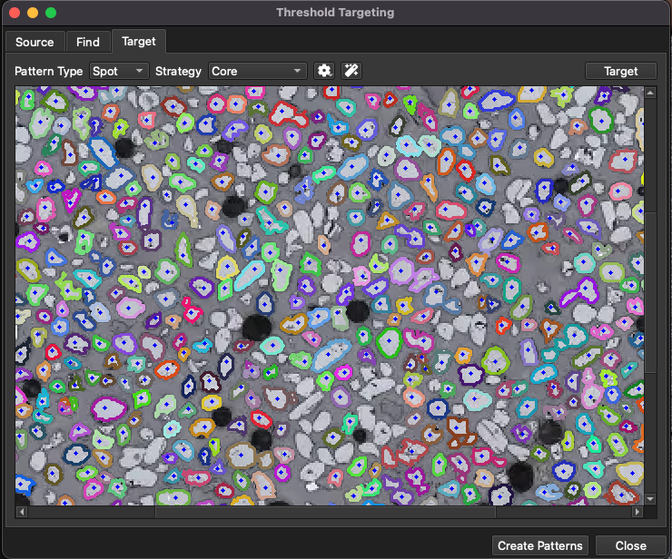
Fig. 14 A screenshot showing the Threshold Targeting window

In this example, a spot will be placed on each grain, so leaving this to the default “Spot” option is sufficient, but if your application included putting a line across each identified area, or if you wanted to cover each identified grain with a lasso pattern, you could use the options in the Pattern Type menu to achieve this.

For Spot type patterns, there are several placement strategies:

Core

Uses a distance transform to place a spot at the maximum distance from any non-grain pixels

Rim

Places a spot near the edge of the grain

Random

Randomly places a spot somewhere on the grain

Core then rim

Places a spot in the core and, if sufficient space, another spot on the rim

Moment

Places a spot in the centroid of the grain area. The centroid in this case is the average of the points defining the boundary.

For regular rectangular or circular grains, the Moment option may be sufficient to place a spot in the center of each grain and the Moment strategy is much faster than the Core strategy. However, consider the case where a grain is an exaggerated hour-glass shape with two larger areas with a narrow join area (e.g. Fig. 15). This may be the natural grain shape (e.g. a crystal with resorbtion embayments) or it could be where two grains are touching. A spot placed in the center of this shape using the Moment option would be in the narrow join region, the location of which is shown by the crosshairs in Fig. 15. If the join area is very narrow, or the spot area very large, there is a risk that it will include some background area. In contrast, the Core strategy would determine the distance to any background pixels (shown as greyscale in Fig. 15 (b) with white being the furthest to, and black being the closest to, background pixels). The Core strategy then places a spot on the furthest distance calculated (shown as grey circles in Fig. 15 (a)).

In this schematic example there are places of equal maximum distance. In this case a spot is placed in the maximum distance area closest to the top left of the image by default (the top grey circle in Fig. 15).

In summary, the Core strategy can reduce the chances of placing spots at the join between grains, at the cost of being slower to calculate.

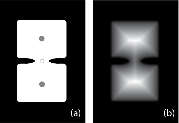
Fig. 15 A schematic example showing wide areas separated by a narrow join. See text for details.

If using the example image, select the Core strategy.

The menu provides options for the chosen strategy. For the Core strategy this is ablation spot size and number of spots to place. For the example image, use a 20 micrometer spot. The button automatically calculates a spot size appropriate for all detected grains. We won’t use it in this case as we want our spot sizes to be exactly 20 µm.

Note

If a spot is too big for the identified shape, no spot will be placed. If many spots are missing, check the spot size.

Click the Target button to place patterns according to the strategy. Depending on the strategy chosen and the number of grains detected, this may take a few seconds.

Click the Target button again if the strategy or settings are changed to regenerate the patterns.

At this point, the patterns have not been added to the region. Click the Create Patterns button at the bottom right of the window to add the patterns to the region. A dialog will appear to enter the root name of each pattern. For example, entering “MySamp” as the root will create patterns with the naming “MySamp_1”, “MySamp_2”, etc. The Create Patterns button does not close the Threshold Targeting window so that you could add different ablation patterns using different strategies without having to detect grains again. After clicking the Create Patterns button, the number of patterns added to the region will be briefly shown in the bottom left of the window. Click the Close button when all patterns have been added.

Properties and Metadata

Expanding the Items Panel (Fig. 16) will now show the patterns automatically created using the thresholding targeting. Selecting ablation patterns in this panel will highlight them on the main image, and show the ablation properties (e.g. spot size, rep rate etc) in the Properties Panel (bottom left of the main window).

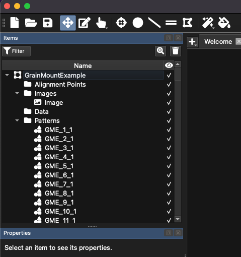
Fig. 16 A screenshot of the Items Panel

The Properties Panel (Fig. 17) shows different properties depending on the item selected in the Items Panel. When ablation patterns are selected, the spot size etc can be adjusted by double-clicking the centre of the spot representation. The colored bar along the bottom of the Properties Panel shows the timing of the selected ablation patterns, with the yellow central band showing the ablation duration, the grey at the start the laser warm up time, and the grey at the end showing the washout time. Double clicking on any of these values shows a dialog to change these.

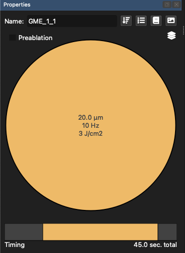
Fig. 17 A screenshot of the Properties Panel

For our example, change the warmup time to 5 seconds by double clicking on the grey area at the beginning of the timing bar, and changing the value to 5 s.

Tip

All patterns within a region can be selected at once using the keyboard shortcut Ctrl + a (Cmd + a on a Mac). Just ensure you have the correct region selected.

Click on the button at the top right of the Properties Panel. This shows the metadata for the selected patterns (e.g. Fig. 18).

Fig. 18 A screenshot of the Metadata window

Ablation metadata include properties of the pattern that are not associated with ablation. Metadata are described in terms of a key (a name for each property, e.g. “area”) and a value. There is one key per property, and a value for each pattern, even if this value is blank. In this example, the keys “area”, “circularity” and “convexity” values from the automated grain finding process, along with the length of the major and minor axis of each grain have been automatically created but custom metadata keys can be created. Keys are shown as columns, and values are shown as cell entries in the Metadata window.

When using ESL systems, the metadata will be added to the LAX file and when the LAX file is loaded into iolite v4, the metadata become properties of the selection. This allows the analyst to plot results calculated in iolite v4 against metadata values, such as grain area. Metadata fields, which are shown as columns in the Metadata window, can be added and removed using the and buttons in the top left of the window.

To add a value to multiple patterns in the Metadata window, select the cells to be adjusted, and click the button in the top left of the window. This will show a dialog where a value can be entered, and that value will be filled in for each row. To enter a value for a single pattern just double-click the cell for that pattern. To clear values, select the cells to be cleared and click the button in the top left of the window. In this example we won’t add any metadata values.

More information about the Properties Panel can be found here.

Adding Alignment Points

For an image to be re-coordinated in laser control software, there needs to be some reference or alignment points. These are typically features that can be identified in both the image and in the laser video output. To set an alignment point, zoom in to a suitable feature using the Ctrl key (Cmd key on Mac) and the mouse scroll wheel, and right-click on the point to be used. Select “Add Alignment Point” to add the alignment point, which are represented as arrows pointing downward in Targeting.

Tip

To pan around the image, ensure the button (top left of main window) is highlighted, and left click and drag.

Repeat this two more times to create two more alignment points. Selecting the alignment points in the Items Panel will show the area saved with the alignment point that will be shown when re-coordinating the region in AV2.

Tip

A screenshot of the main area can be easily created by clicking the button in the top right of the main window. This can be handy when selecting and storing alignment points.

Note

In CSV exports (i.e. for non-ESL systems) only the coords of each alignment point are exported. Metadata is not supported for other systems

A Targeting file can be saved by going to the File menu and selecting “Save As”. Once you have selected three alignment points, save the file.

Adding a blank region

Continuing with our example dataset, we will now add reference material (RM) analyses. Normally, multiple reference materials would be used but for brevity only a single will be added here. The process is the same for multiple RMs.

To create a blank (empty) region, click the button and select Region. A dialog asking for the region name and physical extents will appear. For the example label the region “Plesovice” (a commonly-used zircon reference material) and set the physical extents to 1 mm x 1 mm.

Note

We will not add alignment points for the reference material region. Instead a series of spots will be added and manually moved into position once the experiment is loaded into AV2. This avoids having to know in advance which areas are clear for ablation on the RM mount.

A new empty region will now appear in the tabs along the top of the Main Panel. Click the button in the toolbar and left click to start defining a shape. To finish defining the shape, double-click when adding the final vertex. After the final vertex is added, a dialog will appear showing options for filling the shape (Fig. 19).

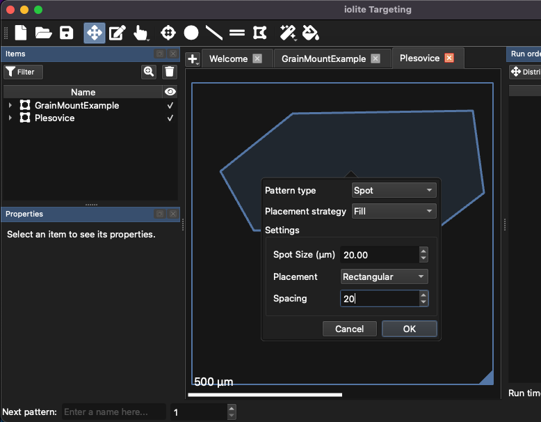
Fig. 19 An example of using the fill tool to create spot patterns

Select “Fill” for the Placement Strategy, and 20 µm for the spot size and spacing. Other settings can be left as default (see Fig. 19). Click OK, and enter a default name for the spot patterns (“Plesovice”).

It’s easy to delete points, so create a shape slightly bigger than you need in this step and delete patterns later.

Spot patterns for the reference material have now been created so we can move on to creating the run list.

Creating The Run Order

Patterns can be dragged individually, or as selections of multiple patterns, to the Run Order List. If the Run Order List is not visible, click the button (top right of main window).

Tip

You can add all patterns in a region to the Run Order List by dragging the region’s Patterns folder to the Run Order List.

Add all spots from the grain mount example region to the Run Order List by dragging the ‘Patterns’ folder to the Run Order List. You may need to expand the region in the Items Panel to see the Patterns folder.

There may be thousands of patterns in the region, and this may be untenable to run in a single session. At the bottom of the Run Order List there is an indication of the approximate run time of the patterns in the run list. To reduce the number of patterns in the run list, select patterns and click the button. This button randomly sub-samples the selected patterns. After clicking the button, enter the number of patterns required after sub-sampling.

Tip

Because the sub-sampling process is random, there is no potential bias towards grains of a particular size, shape or appearance beyond the settings entered in the automatic targeting process.

Alternatively, selecting patterns in the list and clicking the button (top right of Run Order List) will remove the patterns from the Run Order List. The patterns will not be deleted from the region, so that they can be added again later if needed.

Select all the grain mount example spot patterns by clicking on one pattern in the Run Order List and pressing Ctrl + a (Cmd + a on Mac). Click the button to sub-sample the list to 1000 patterns.

Add the reference material (“Plesovice”) spot patterns to the Run Order List by dragging the ‘Patterns’ folder from the ‘Plesovice’ region to the top of the Run Order List. Select all the Plesovice patterns in the Run Order List, and distribute them so that a Plesovice spot is run every 30 minutes by clicking the Distribute button, selecting the ‘by time’ option and entering 1800 s (= 30 minutes). A Plesovice spot will now be run every 30 minutes.

Depending on the size of the area filled in the previous step, you may have excess Plesovice runs at the end of the Run Order List. Delete these by scrolling to the last Plesovice run needed, and select the excess and clicking the button at the top right of the Run Order List.

This process can be repeated for other reference materials.

The experiment is now ready for export.

Exporting the Run List and Metadata

To export the patterns as an LAX file, with all the images and metadata saved within, ready to be re-coordinated in AV2, to the File menu and select Export to LAX. In this example, our Plesovice region does not have alignment points as the spot patterns will be moved to a clear area(s) when loaded in the cell. Click Yes to continue. Select a location and file name for the export and click OK. The LAX file will be created and can be transferred to the AV2 computer when it is time to run the experiment.

To Export to a CSV (comma separated values) file, go to the File menu and select Export to CSV. No images or metadata will be saved with the csv file.

Importing the LAX file in AV2

Once the LAX file created by Targeting has been transferred to the AV2 computer, start the laser and AV2 as per normal operating instructions. Once set up, click ‘Open Experiment’ from the File Management Tab and select the LAX file created by Targeting. A re-coordination wizard will appear (Fig. 20).

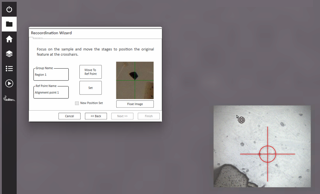
Fig. 20 The re-coordination wizard in AV2

For each region within the LAX file, the re-coordination wizard will guide you through selecting the alignment points in AV2.

Tip

An image of the holder after samples have been loaded can be useful when running the re-coordination wizard. Similarly, screenshots created in Targeting can help with re-coordination. Alternatively, Sample Maps (camera image mosaics) can be useful in finding alignment points. Sample Maps are created using the Sample Maps tool (globe icon in the Tools section, lower right hand of AV2 window).

A snapshot from Targeting of each alignment point is shown in the re-coordination wizard. This snapshot can be floated by clicking the ‘Float image’ button.

Drive to the alignment point, and ensure that the position (x, y values) and focus (z value) are accurately set. Click the Set button in the re-coordination wizard, and click ‘Next >>’’ to move to the next alignment point. Repeat for the next two alignment points. When all three alignment points have been set click Finish. The images and patterns from the LAX file will be re-coordinated and available for ablation in AV2.

The experiment is then ready to run.

Example 2: Image Region Targeting

In this demonstration, the example image is an SEM image with embedded coordinate information. Targeting can read this information automatically and scale the image appropriately. To follow along with this example, download the tiff image here. Import the image using the button or using the keyboard shortcut Ctrl + i (Cmd + i on Mac). As this image has embedded spatial information, the Scale option should automatically be “Embedded Information”. Leave the Import Type as “Region” to create a new Region and click OK. Leave the Region name as the default provided and click OK.

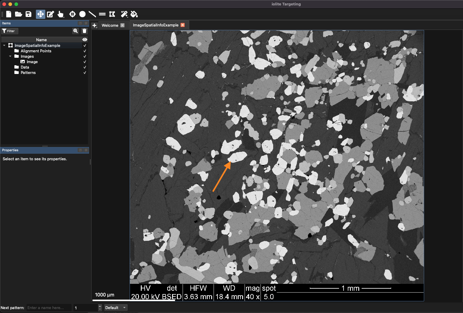
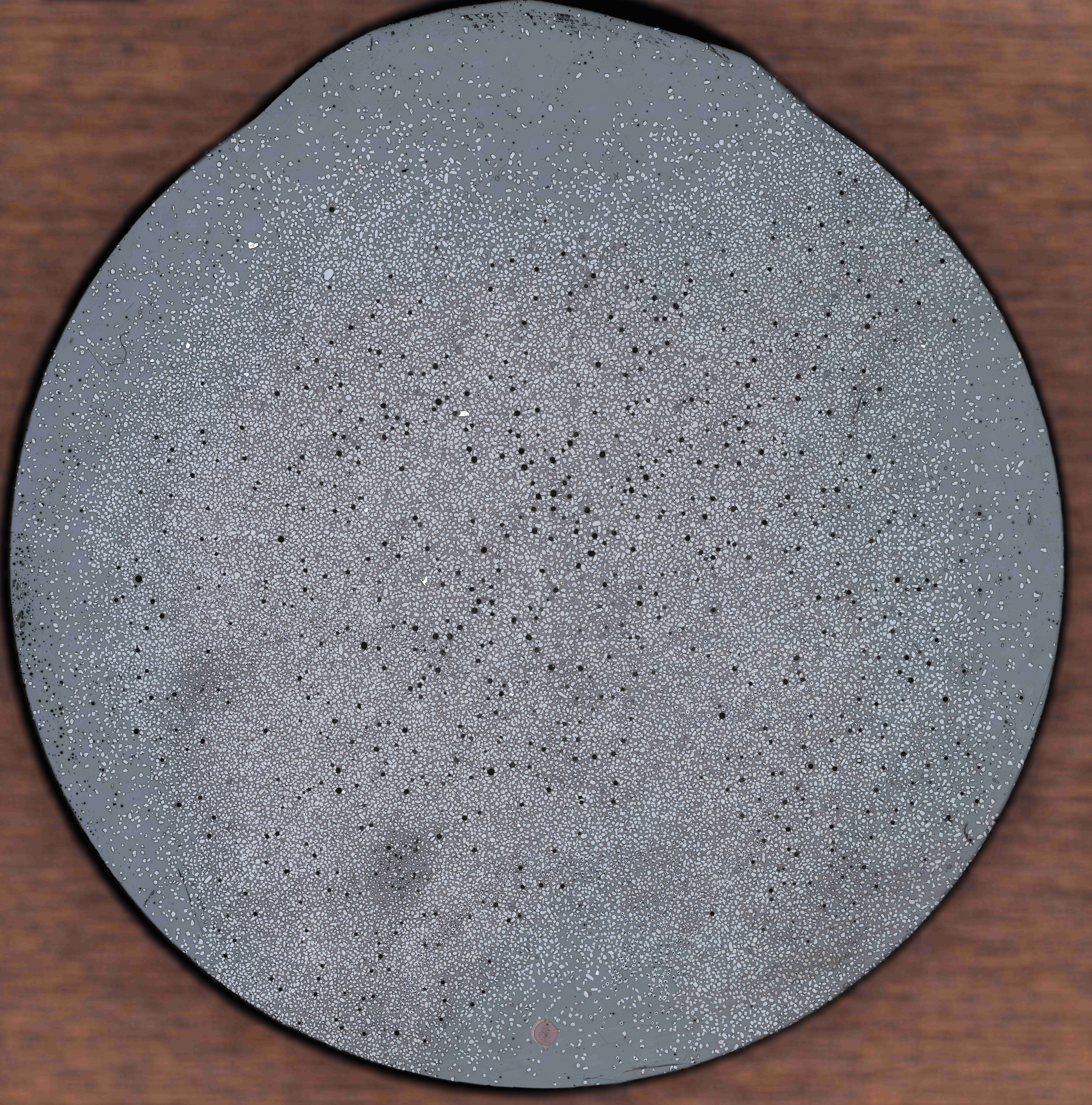
Fig. 21 The example image with embedded spatial information. The orange arrow highlights one of the grains described in the text.

There are basically four different phases in this image varying from very dark grey to light grey. For this example, we will target some of the light grey regions for additional imaging analysis. An example of a light grey grain is included in Fig. 21 but any grain would work. Zoom in to one of the light grey grains using Ctrl + scrolling the mouse wheel.

Tip

Keep the mouse cursor over the area you want to zoom to while scrolling. This will avoid it going off screen and make it easier to zoom to the selected area.

When zoomed in on one of the light grey areas, right click in the area and select ‘Fill Segment’ from the right-click menu. This will automatically select pixels in the image using a flood fill algorithm. This selects pixels surrounding the pixel clicked if they are similar in value. The area determined by the flood fill algorithm will be outlined by a blue line, and options for filling the area will be displayed.

In this case, we want to create an imaging lasso pattern, so from the Pattern Type menu, select Lasso. The only Placement Strategy for a Lasso pattern type is ‘Cover’ so that can remain unchanged. The options for a lasso fill are: spot size, buffer and epsilon values. The buffer value determines how much to enlarge the polygon before filling with lines. This can be useful to include some surrounding area around the area of interest. The units for the buffer value are in micrometers. Epsilon determines how much the shape should be simplified. A larger epsilon value means more simplification (i.e. the resulting polygon has fewer points and less detail), while a smaller epsilon value keeps the shape closer to the original.

Change the spot size to 10 µm and the buffer to 20 µm and click OK. Enter a name for the lasso pattern when prompted.

You can change the ablation properties, as described in Properties and Metadata section, however because this is a lasso pattern, there are now properties for the overlap and line spacing. Adjusting the former automatically updates the scan speed to match the overlap value. Change the line spacing to 10 µm, set the overlap to 3 µm, and change the spot shape to square using the buttom at the top right of the ablation properties panel.

This process of using the flood-fill algorithm for targeting can be repeated for several more areas. After all required areas have been assigned ablation patterns, the experiment is ready to be finished up with alignment points and reference material patterns as described for the previous example, starting at Adding Alignment Points.

Example 3: Loading point data files

This example demonstrates how to load point files associated with an image, and uses the same image as the previous example. If you don’t have it open, follow the instructions in the first paragraph of the previous example.

In this case, we’ll be loading some SEM point analyses in a .dat file but Targeting supports Excel, csv, txt and dat files. You can download the example .dat file by right-clicking here and selecting “Save Link As”. Leave the filename as suggested by your browser.

Import the points file by clicking the button and selecting ‘Data’. Select the example file and open it. The Data Import window will appear (Fig. 22).

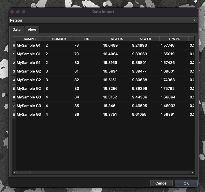
Fig. 22 The Data Import window in iolite Targeting

At the top of the Data Import window there is the Region dropdown menu. If it is set to ‘Region’ a new region will be created for the data file. In this example we want to use the data file with the image already imported, so change the region option to ‘Data in Region’.

There are two tabs below the Region dropdown menu: Data and View. Use the Data tab to see the values that will be imported. If you scroll to the far right of this tab you’ll see that this file has x and y columns labelled ‘X-POS’ and ‘Y-POS’.

Click on the View tab to see how the points plot in x,y space. In this example, Targeting has automatically chosen the X-POS and Y-POS columns for the x and y data, but clicking on the dropdown menu beside the X and Y labels allows you to choose which columns to use for the x,y coordinates. Targeting will store the names selected for future imports.

Because these data points are being loaded into an existing region, you need to establish the mapping between the current coordinates of the point data and the underlying region. You can do this using the three landmarks approach. Click on a data point in the View Tab (in the Data Import window) and click on a corresponding point in the underlying region. In this example, it doesn’t matter how you place the points, but Fig. 23 shows an example placement. Just make sure that for each point you click in the Data Import window first, then in the Main Panel. If you make a mistake, click the Reset button at the bottom left of the Data Import window to start again. Click OK to import the points into the region.

Tip

Just like in other parts of Targeting, you can zoom in and out in the View tab by holding Ctrl (Cmd on Mac) and scrolling the mouse wheel. This can improve the accuracy of the alignment process.

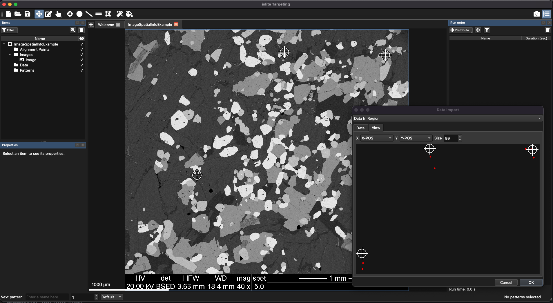
Fig. 23 An example of placing points in a region using the three landmarks approach. The crosshairs in the Main Panel correspond to points in the Data Import window.

After the points have been placed in the region, they will appear in the Data sub-folder in the Items Panel and will be plotted in the Main Panel. If a mistake was made during the alignment process, the points can be deleted by selecting them in the Items Panel and pressing the Delete key, then importing them again using the same process described above.

To adjust how the points are displayed, select them in the Items Panel, and adjust their size by entering a value in the Size field (50 be default) in the Properties Panel. Change the color of the points by clicking the … button in the Properties Panel.

Coloring and scaling points by properties

Although this is a small dataset, it can be useful to adjust how the data points are displayed so that points of interest can be targeted easily. A basic way of doing this is to color the points by the one of their properties. Each column in the data file is imported as a property. To color the points by a property, make sure all points are selected in the Items Panel and in the Properties Panel click the dropdown menu next to Color. This will show all the properties of the data points. Select FeO from the properties. The points are now colored by FeO value and one of the lower left points stands out as having higher FeO while the three points in the top right have lower FeO values. To change the color scale applied, click the Gradient dropdown menu and select a different gradient. To see the upper and lower limits of the gradient, click the Show button.

To scale the size of the points by a property, select a property from the Size dropdown menu. Select FeO again. It is now visually very easy to pick spots based on their FeO content, but any property could be used for scaling and coloring data points.

To remove scaling and coloring of points by a property, select the first entry in the dropdown menu, which is a blank value. This will reset points to their default color and size. Reset the example points before proceeding.

Filtering items by property

The scaling and coloring of datapoints above is a fast qualitative approach to finding points of interest. A more refined approach is to use filtering. At the top of the Items Panel is the ‘ Filter’ button. This button shows/hides the filter controls at the top of the Items Panel. Filtering can apply to any item, but in this example will be applied to the imported data points.

Select all of the data points in the Items Panel, and click the Filter button to show the filter controls. You can add/remove filters by clicking the or buttons, respectively. Add a filter now by clicking the button. Each filter consists of an Attribute (a property to filter by), a Comparator (such as equal to, greater than, etc) and a Value for comparison. When you add a filter the Attribute is empty, the Comparator is ‘=’ and the Value is empty.

Double-click in the Attribute field to add an attribute to filter by. Type “data.” to show a list of properties for the data points. Keep typing to narrow the choices presented. In our example we’ll filter by ‘Na WT%’. Type “data.Na” and select “data.Na WT%” using the arrows keys and press Enter to select it.

Tip

If typing ‘data.’ does not show any suggestions, make sure you have your data points selected in the Items list.

Change the comparator by double-clicking it (the default value will be ‘=’). Change it to greater than (‘>’). Double-click in the Value field and set the value to 0.1. The list of data points will now show only points 1, 3, 5, 6, and 7, as these data points have greater than 0.1 Na wt%. The ‘Hide’ button at the top hides any items not matching the filters in the Main Panel. Click it to show only the points matching the Na wt% filter.

To show points that have values within a defined range, select the ‘in range’ comparator, and enter the lower and upper values like so ‘[lower],[upper]’. For example, to select points with Na wt% values between 0.05 and 0.1, enter ‘0.05,0.1’ in the Value field.

Additional filters can be added by clicking the button. For an item to appear in the list it must match all filters unless the ‘Any’ button (top right of filter controls) is selected. If this option is selected, items matching any filter will be shown.

Try adding two criteria: Na WT% in the range 0.05 - 0.1, and Si WT% less than 16.4. Only two points should match those criteria: points 8 and 9. If you see more than this, ensure that the ‘Any’ option is not selected.

Remove all filters by clicking the button before proceeding.

Patterns can also be sorted in the Items Panel by clicking the button in the Properties Panel. This will prompt the user for a property to sort by. By default, items in the Items Panel are sorted by ‘name’. In this example, try sorting by x position by clicking the button and entering ‘x’ as the property to sort by. The updated order should be Spot 4, 5, 6, 1, 2, 3, 7, 8, 9. To return to the default ordering, select all patterns, click the button again and enter ‘name’.

Creating ablation patterns from data points

To create ablation patterns from data points, select the data points in the Items Panel and click the ‘Create Patterns’ button in the Properties Panel. A spot pattern will be added for each selected data point.

Note

Ablation patterns can be filtered in the same way as data points in the previous section.

Try filtering the ablation patterns by adding a filter ‘x’ > 1700. Only patterns 1,2,3,7,8 and 9 should match the criteria. In this way, ablation patterns within a certain part of a larger region could be selected by x,y position.

Tip

The x,y coordinates of a pattern is shown in the bottom right of the main window.

Remove all filters by clicking the button before proceeding.

Copying metadata to ablation patterns

As discussed in the Properties and Metadata section, metadata for ablation patterns were introduced. To briefly revise, metadata are data related to the ablation patterns. This could include anything, such as sample IDs, field trip labels, or compositional data collected by another technique. Metadata stored with patterns in Targeting are passed through AV2 to become available in iolite. This could be used to help process the data in iolite (for example, major element contents measured by electron microprobe could be used as internal standard values) or even for storage in databases (for example, storing a project ID so that all samples assigned to a project can be easily found within a database).

In this example, the SEM data points contain major element information recorded by the SEM. Our aim is to include these values as metadata for the spot ablation patterns. To do this, select all spot patterns in the Items Panel (the shortcut key is Ctrl + a to select all patterns in the current region) and open the Metadata Window by clicking the button in the Properties Panel (top right). By default the spot patterns will have no metadata values. Click the ‘From Items’ button in the top right of the Metadata window. Targeting will find any other items overlapping with each pattern in the Metadata window.

In this case, the patterns overlap with the data points so the properties of each data point will be copied across as metadata to the ablation pattern. In addition, the patterns also overlie the background SEM image, so the RGB value of pixels overlapping with the spots will be recorded, labelled as ‘Image_r’, ‘Image_g’, ‘Image_b’ and ‘Image_gray’ in the metadata columns. This feature could be useful, for example, where the color of the image may relate to some physical property not recorded elsewhere such as intensity in cathode luminescence images which could be compared to U-Pb ratios in iolite v4.

The ablation patterns now have a full complement of metadata, and at this point, alignment points could be added to the region, and a run order list established. These concepts are covered in the first example, starting at Adding Alignment Points.

This concludes this example showing how to import data points, as well as demonstrations of applying filters to items and metadata collection in Targeting.

Example 4: Loading maps from iolite files

This example shows how to load an image from an iolite file and select targets for image lasso regions. A possible scenario for this approach is an experiment where an initial reconnaissance LIBS map has been created of the entire sample to identify areas for further analysis. This can be helpful to identify features not obvious to the naked eye or are not visible in images previous collected using other techniques.

The example dataset in this example is too large to share, however the steps are the same for any LIBS or LA-ICP-MS experiment processed in iolite. In this example, a rapid LIBS map was collected of a very large (approx 440 x 470 mm) sample. The data were processed in iolite, including image creation and principal component analysis. In iolite, the principal components can be plotted as images similar to any other channel. In this example, the first principal component identifies the areas we would like to target so the PCA_1 map will be imported into Targeting.

Click the button at the top left of the Main Panel, and select ‘iolite’ to import an image from an iolite experiment (.io4) file. Targeting will read the .io4 file, and provide options for which group and channel to import (Fig. 24). In this example, we’ll select our sample group and the PCA_1 channel. The other import settings can be left as default, but if your image was created using the traditional (i.e. not CellSpace) approach, this option can also be selected from the controls at the top.

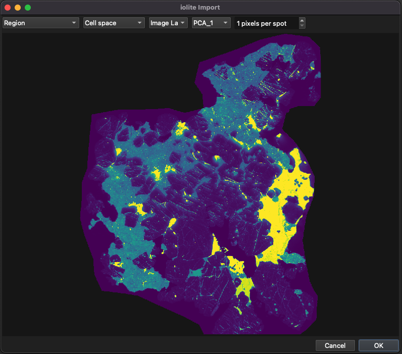
Fig. 24 An example of importing an image from an iolite v4 .io4 file

The image will be imported and can then be used to target areas as described in Example 2: Image Region Targeting where the flood fill algorithm was used to select areas for more detailed analysis.

Example 5: Using Targeting’s Trainable Segmentation Feature

This example uses Targeting’s trainable segmentation feature to break an image up into “phases”. We use the term phases here instead of “minerals” etc as it is a more generic term. Depending on the sample, phases could represent different tissue types, areas of staining etc. The base image for this example is the SEM image from Example 2: Image Region Targeting: there is a download link that example. Download and import it using the steps described in Example 2.

Example 6: Using Precognition for improved imaging experiments

Precognition is a tool for highlighting possible issues with imaging experiments. In particular, it can help identify when the laser settings are inappropriate for the mass spec settings. It also creates a predicted image to indicate the level of detail that may be possible gniven a set of laser and mass spec settings.

How it works

Precognition uses the laser pattern information, along with the modelled cell response and a base sample image, to generate time series data. These time series data are sampled according to the mass spectrometer’s acquisition parameters, and the result is input into iolite’s image generation algorithms to create a predicted image. The base image can be any image of the sample such as a photomicrograph or SEM image etc, but should be at sufficient resolution to see the features of interest without being excessively detailed or an excessively large image file. It is important to note that the prediction is not trying to model what the trace element distributions will be exactly, but to give the analyst a sense of what level of detail would be available if the current analytical settings were used.

Precognition will also provide warnings if it identifies potential issues with the analytical parameters. These include image aliasing (frequency effects between the mass spec sampling frequency and the laser ablation rate); issues with the laser or mass spec settings (e.g. scanning the laser too quickly, or insufficient dwell time for low signal to noise elements); as well as providing overall information about the experiment such as spot overlap, pulse dosage and total analysis time.

General Workflow

The general workflow is to import any imagery for your experiment, and to create imaging patterns (raster or lasso patterns).

Tip

Lasso patterns can be changed to “image mode” in Targeting’s preferences, in the Other section.

To use Precognition the predict the measurement results of an ablation pattern(s), you must first set up:

1. A laser pulse profile, and

2. A mass spec setup.

Precognition will use the pattern information, such as rep rate, spot size, and scan speed, along with the mass spec setup, such as the counts for each element (m/z) and the dwell times, along with the underlying image to predict what the result of measuring that pattern would be if the pixel intensity in the underlying image represented the concentration of the selected element.

Laser Pulse Profile

A laser pulse profile is a model of the mass spec’s response to a single pulse from the laser. Adding a profile will present the pulse profile edit window (Fig. 25).

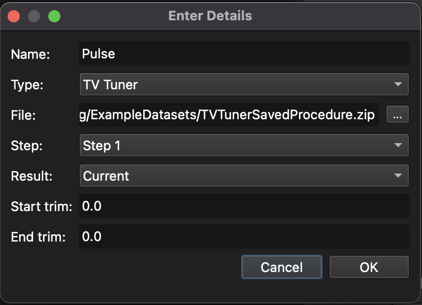
Fig. 25 The laser pulse profile edit window

The laser pulse response can either be provided as a file if it has been measured, or described by some mathematical equation describing the signal (e.g. ).

If the Model option is chosen, the pulse duration and the time resolution (i.e. the number of data points to use to model the pulse response) can be set, along with the expression. The expression is a python expression and takes a variable for the time. Any numpy functions (e.g. exp(), power()) can be called without a prefix (e.g. “np.exp()” or “numpy.exp()” is not required).

If the File option is chosen, a file containing time and intensity values can be selected and loaded for the profile. The file can be a comma-separated values (.csv); Excel file, where the first column is the time values, and the second column is the intensity values, with no header row; or, a JSON file, created by exporting an existing pulse file (see below). To select the file, click the … button next to the File field. Values can be trimmed from the start and end of the file using the “Start trim” and “End trim” fields.

If the TvTuner option is chosen, a zip file created by the TvTuner plugin for AV2 can be chosen. This zip file should be the results of single pulse response (SPR) tuning, and Targeting will read the file and extract pulse response. The zip file can be created in TvTuner by clicking the “Create zip” button in the Action panel at the bottom of the TvTuner panel. If the Procedure in TvTuner had multiple Steps, the step can be chosen with the Step field, along with the Result (see here for full TvTuner documentation). The Start and End trim fields can be used to trim the start and end values from the TvTuner file.

Several different pulse profiles can stored, each with their own name (settable in the Name field, or by double-clicking the name). You can export a pulse by clicking the button. This will save the pulse to a .json file that can be shared with others (e.g. iolite support, etc).

Mass Spec Setup and Analytes

A “Mass Spec Setup” is a series of “Analytes” used by Precognition to model how a laser signal might be recorded by a mass spec. Each Analyte typically represents an element (a single m/z) and has a series of values, such as background, sensitivity, dwell time, etc, that affect its measurement, and are used by Precognition to determine what an image of each Analyte might look like. To create a new Mass Spec Setup, go to the Analytes tab in Precognition’s preferences, and click the button on the left hand side. This will create a new setup and ask for the name of the setup. Initially the Setup has just a single Analyte (U238). Clicking the Setup in the list (on the left hand side of the window) will show the Analytes.

To add an Analyte, click the button in the middle of the window. This will add a new Analyte to the table of Analytes that takes up most of this window. Each Analyte has the following properties:

• Name (can be anything)

• Mass (m/z)

• Dwell time (the amount of time spent measuring this m/z each measurement cycle)

• Settle time (the amount of time spent moving to this mass, typically a non-adjustable value from the mass spec)

• Peak (the sensitivity of the element, usually determined on a reference material, in counts per µg.g-1)

• Background (the background counts)

• Flicker (the amount of noise to be added, as a percentage, which is used by Precognition to mimic counting noise)

Double click on any of these properties to adjust them.

To remove an Analyte, click the button.

To automatically import values from an existing iolite .io4 file, click the button. This will allow you to select a .io4 file, and then ask which selection group best represents the sample you’d like to analyse by Precognition. It will also ask for a group representative of the baselines (typically a baselines selection group). It will then automatically create the Analytes measured in the file, and fill in the sensitivity etc for each Analyte.

Tip

If you don’t know what sensitivity etc to expect, it can be helpful to measure a sample similar to the sample you want to predict for, or to measure a part of the sample not in an area of interest to gain more accurate estimates of the backgrounds, sensitivities etc.

Analysis Optimization

Precognition offers three optimisation strategies for optimising the dwell times for each analyte. These are ‘Hutchinson’, ‘van Malderen’ and ‘Even’.

Hutchinson method

The Hutchinson method attempts to reduce the dwell times while maintaining the statistical difference between the background and peak signal, given the current analyte background and peak counts and dwell times. For example, if you have an analyte with significant difference between the peak and background, you may be able to decrease the dwell time to reduce your overall cycle time. You can set the number of standard deviations between the peak and background using the Sigma parameter. You can also add additional ‘breathing space’ between the two populations (peak and background) using the ‘Breathing space’ parameter. As this method aims to reduce the dwell time based on the observed counts, it may reduce the dwell times to values that result in very low duty cycle (the amount of time spent collecting data relative to the total cycle time). You can avoid this by setting a minimum dwell time. For more than one or two analytes, we would recommend dwell times of no less than 10 ms. If your mass spec allows setting fractional dwell times, you can check the fractional dwell times checkbox to avoid having to use whole millisecond dwell time values. However, this may result in dwell times just slightly lower than the specified minimum dwell time.

To avoid frequency effects between your laser firing rate and your mass spec cycling time, you can choose to synchronize your total cycle time with some multiple of the laser repetition rate using the ‘Synchronize cycle time to rep. rate’ checkbox. If this value is set to one, the optimisation will attempt to fit all masses between one pulse of the laser and the next. If this results in very short dwell times where the mass spec duty cycle is too low, you can expand the number of cycles using the Cycles parameter. For example, by default this parameter is 1 and all masses will be fit into one laser pulse. Increasing this to 3 will fit the total cycle time into three pulses of the laser, allowing for longer dwell times and more reasonable duty cycles.

van Malderen method

The van Malderen method distributes the dwell times within the total cycle time according to the inverse of the signal to noise ratio (SNR) of each analyte. You can set how many pulses of the laser the total cycle time should be synchronized with using the ‘Synchronize cycle time to rep rate ‘ checkbox, and you can set the minimum dwell time using the ‘Minimum dwell time’ parameter.

Even method

This method simply distributes the dwell times for all analytes evenly within the total cycle time, while synchronizing with the laser repetition rate. You can set the number of cycles to synchronize with the laser pulses, as well as the minimum dwell time.

Note

After you have run an optimisation, the background and peak count rates and flicker values displayed in the analytes table will no longer reflect what would be expected from a measurement with the displayed dwell times. That is, if you have decreased your dwell times you may have also increased your uncertainty for both background and peak count rates. You should not run another optimisation until you have measured another test scanline using the suggested dwell times to update the background and peak values.