Image Processing in iolite Targeting

Images that can be used for targeting in iolite Targeting include SEM images, CL images, BSE images, and any other image type that can be imported as a PNG, JPEG, TIFF or BMP file. Images can be imported into Targeting using the button in the Main Window documentation.

However, images may require some processing to optimize them for targeting. This might include applying filters to enhance edges or features of interest, or removing mosaic effects. The various image processing options available in iolite Targeting are described below. All options are accessed by right-clicking on the image in the Items Panel and selecting “Image Processing…” from the context menu. This opens the Image Processing panel (Fig. 7).

For all image processing operations, the original image is preserved and a new processed image is viewable using the “Original” and “Corrected” buttons in the top right of the Image Processing panel. To replace the source image with the corrected image, check the “Replace source” checkbox at the bottom left of the panel. If this is not checked, a new image will be added to the region when the Save button is clicked (bottom right of the panel).

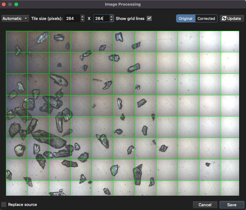
Fig. 7 Example of the Image Processing Panel in iolite Targeting

Clicking the Update button will apply the selected image processing operations to the original image. The processed image can then be viewed in the “Corrected” view.

Note

It may be necessary to apply one or more operations to make an image suitable for targeting. For example, applying a mosaic correction and then a background correction.

Images in the Image Processing panel can be zoomed and panned using the mouse. Use the mouse wheel + Ctrl Key (Cmd Key on macOS) to zoom in and out. Left-click and drag to pan the image.

Adjusting Contrast

The following contrast adjustment options are available:

Simple scaling

A simple scaling operation between a min and max value to adjust the overall brightness of the image. Pixel values below the min value will be set to 0 (black), and pixel values above the max value will be set to 255 (white). Pixel values between the min and max values will be linearly scaled between 0 and 255.

Linear Contrast

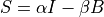
Adjusts the contrast of the image linearly by stretching the histogram of pixel values. It does this by applying the following equation:

$\mathrm{output\_value} = \alpha \cdot \mathrm{input\_value} + \beta$

where $\alpha$ is the contrast factor and $\beta$ is the brightness offset. Increasing $\alpha$ increases contrast, while increasing $\beta$ increases brightness. $\beta$ can also be a negative value to decrease brightness.

Note that output pixel values are clipped to the valid range (e.g., 0-255 for 8-bit images).

Histogram Equalization

Enhances the contrast of the image by redistributing the pixel intensity values. This has the most effect when the image has a narrow range of intensity values.

CLAHE (Contrast Limited Adaptive Histogram Equalization)

Improves local contrast and enhances the definition of edges in each region of the image. Adjust how many parts the image is divided into using the “Grid Size” parameter. A larger grid size means more parts and more localized contrast enhancement. The “Clip Limit” parameter controls how much contrast enhancement is applied. A higher clip limit allows for more contrast, while a lower clip limit limits the contrast to avoid noise amplification.

This method is particularly useful for improving the visibility of features in images with varying levels of brightness across different regions of the image.

Gamma Correction

Adjusts the brightness of the image using a non-linear transformation, using the formula:

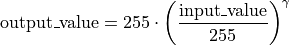
$\mathrm{output\_value} = 255 \cdot \left(\frac{\mathrm{input\_value}}{255}\right)^{\gamma}$

where $\gamma$ is the gamma value. A $\gamma$ value less than 1 will make the image appear lighter, while a $\gamma$ value greater than 1 will make the image appear darker.

See this webpage for an example of gamma correction: Gamma Correction Example.

Applying Smoothing

The following smoothing options are available:

Box
Gaussian
Median
Bilateral Filter
Low pass filter
Wavelet
Non-local Means

Box Blur

Applies a box blur to the image, which smooths the image by averaging pixel values in a surrounding neighborhood. The size of the neighborhood can be adjusted using the “Size” control.

Gaussian Blur

Applies a Gaussian blur to the image, which smooths the image by averaging pixel values with a Gaussian kernel. The size of the kernel can be adjusted using the “Size” control and the number of standard deviations can be adjusted using the “Sigma” control. A larger feature size will result in a more blurred image, and a larger value of Sigma will result in a more pronounced blur effect.

Median Blur

Applies a median blur to the image, which replaces each pixel value with the median value of the pixel values in a surrounding neighborhood. The size of the neighborhood can be adjusted using the “Size” control. A larger feature size will result in a more blurred image.

Bilateral Filter

Applies a bilateral filter to the image, which smooths the image while preserving edges. It takes into account not just the distance to other pixels, but also the intensity values. The size of the neighborhood can be adjusted using the “Diameter” control. The “σColor” value can also be adjusted to change the amount of smoothing, and the “σSpace” value can be adjusted to change the amount of spatial smoothing.

Low Pass Filter

Applies a low pass filter to the image, which smooths the image by removing high frequency noise. The “Cutoff” control can be adjusted to change the cutoff frequency of the filter. A lower cutoff frequency will result in a more blurred image. The “Order” control can also be adjusted to change the steepness of the filter roll-off. A higher order will result in a steeper roll-off.

Wavelet

Applies a wavelet transform to the image, which can be used to denoise the image.

Non-local Means

Applies a non-local means filter to the image, which smooths the image by looking for other areas of similar pixel values. The size of the areas can be adjusted using the “Size” control, and the “Distance” control can be adjusted to change how far the alogorithm looks for similar areas.

Removing Background

There are two options for removing backgrounds from images: “Automatic” and “Manual”.

The manual option allows you to click on the image to specify areas of background. The size of the areas can be set using the “Feature size” control. The larger the feature size, the larger the areas that will be selected as background. After clicking on the image to select background areas, click the “Update” button to apply the background removal. A surface representing the background will be interpolated from the selected areas and subtracted from the original image.

The automatic option downsamples the image and converts it to grayscale (if it was color to start with). It then applies a Gaussian blur to smooth the image and determine the average intensity. The original image intensity is then divided by the smoothed intensity, and the image is converted back to color (if required). Dividing by the smoothed intensity has the effect of normalizing the image intensity.

The size of the Gaussian blur can be adjusted using the “Feature size” control. A larger feature size will result in a smoother background mask, but a smaller feature size may increase the presence of noise in the image.

Correcting for Mosaic Effects

Mosaic effects can occur in images that are created by stitching together multiple smaller images. This can result in visible seams or differences in brightness or color between the different sections of the image. The mosaic correction option attempts to correct for these effects by adjusting the brightness and color of the different sections.

Note

This option assumes that the mosaic is regularly arranged in a grid pattern. It will not work well for irregularly arranged mosaics (e.g. offset rows etc).

The size of the sub-images (tiles) can be adjusted using the “Tile size” control, which should match the size of the visible tiles in the image.

There are two options for the correction method: “Automatic” and “Manual”. The manual option allows the user to click on tiles to specify areas that should represent a uniform background (i.e. areas free from sample grains; areas of clear glass or epoxy, etc). These areas are used to define the uneven illumination of each tile. The algorithm samples the average intensity of the selected tiles and adjusts the brightness and color of the other tiles to match. After clicking on the image to select background tiles, click the “Update” button to apply the mosaic correction.

The automatic option downsamples the image and converts it to grayscale (if it was color to start with). It then applies a Gaussian blur to smooth the image and determine the average intensity. The original image intensity is then divided by the smoothed intensity, and the image is converted back to color (if required). Dividing by the smoothed intensity has the effect of normalizing the image intensity.

Edge Enhancement

This option provides a simple way to enhance edges in an image using unsharp masking. Edges are detected by comparison between a smoothed and unsmoothed version of the image. The enhanced image $S$ is calculated as:

$S = \alpha I - \beta B$

where $I$ is the original image, $S$ is the smoothed image, and $B$ is a Gaussian blurred version of the original image. The amount of blurring is set using the Radius control, with $\alpha$ and $\beta$ as scaling factors that control the amount of edge enhancement set using the “Alpha” and “Beta” controls.

Texture Detection

The texture detection highlights areas of the image with high local contrast, which can be useful for identifying features in images with low overall contrast. The “Footprint” control sets the size of the local area used to calculate the local contrast. A larger Footprint size will result in a smoother texture map, while a smaller feature size will result in a more detailed texture map. Areas of high complexity (e.g. edges, grain boundaries, etc) will appear bright in the texture map, while areas of low complexity (e.g. uniform areas of glass or epoxy) will appear dark.

Masking

The masking tool fills areas of similar color with a uniform color. This can be useful for defining backgrounds as a single color to make feature recognition easier.

The process involves clicking areas on the image to define areas to be considered similar such as the background. When the Update button is clicked, the selected areas will try to expand as much as possible (according to the algorithm) to fill areas of similar color. The “Size” control sets the size of the area used to determine similarity. Left click on the image to add an area. Left click an area again to remove it. The “Smoothing” control adjusts how much the edges of the masked areas are smoothed. A higher smoothing value will result in smoother edges, while a lower value will result in edges. This can affect how well the masked areas fill in gaps.

The color used to fill the masked areas can be set using the color picker next to the “Smoothing” control. Click on the color box to open a color selection dialog.

It may be necessary to run the process multiple times to ensure that all areas of similar color are filled. If areas are missed, simply left click on those areas to add additional areas and click the Update button again. Normally within a few iterations the entire area of similar color will be filled.

Conversion to Grayscale

This option converts a color image to grayscale.

Color Inversion

Inverts colors according to a bitwise NOT operation. For example, black (0) becomes white (255), and white (255) becomes black (0). RGB colors are inverted according to the formula: R’ = 255 - R, G’ = 255 - G, B’ = 255 - B. This can be useful for enhancing contrast in some images.

Image Resizing

A common image processing operation is to resize images. This is particularly useful when working with very large images that may slow down performance. Resizing can be done while maintaining the aspect ratio to avoid distortion.

There are two options for resizing images in iolite Targeting: “Pixels” and “Percentage”, where the former allows you to specify the exact pixel dimensions, and the latter allows you to specify a percentage of the original size. This option is selectable using the dropdown menu in the top left of Image Processing panel.

The “Keep Aspect” option maintains the original aspect ratio of the image when resizing. If this option is checked, only one dimension (width or height) needs to be specified, and the other dimension will be automatically calculated to maintain the aspect ratio.

If the new dimensions are larger than the original image, the image will be upscaled using interpolation. If the new dimensions are smaller than the original image, the image will be downsampled using averaging.