Main iolite Targeting Window
The Targeting Main Window displays regions in the main panel, along with the run list and the Regions and Properties panels (Fig. 2). Each region is shown in a separate tab in the Main Panel. Each part of the Main Window is described below.
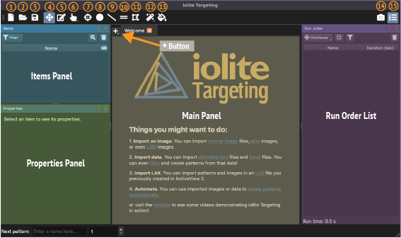
Fig. 2 Annotated screenshot of iolite Targeting Main Window. The buttons are detailed below under Toolbar Buttons
Items Panel
The Items Panel is an organized, expandable list of regions and sub-items. A region typically represents a grain mount or thin-section, and most experiments will have several regions. A key feature of a region is that after re-coordination, the relative distances and angles between lines in the region remain the same, even with some amount of rotation and scaling applied. An example showing this is shown in Fig. 3. Note that multiple grain mounts would not be processed as a single region as after loading in the cell, each grain mount might be rotated by a slightly different amount, which would violate the principle of conserved angles and relative distances.
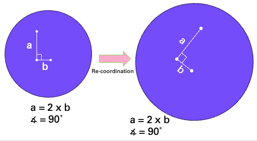
Fig. 3 A diagram showing an example region representing a grain mount with three points for ablation. After re-coordination, the relationship between distances and angles remains the same for the region.
Regions can contain any of the following sub-items: images, data points (e.g. from an SEM point analysis file), alignment points, and ablation patterns. A region can have multiple images which may come from a variety of sources (e.g. SEM, CL images etc).
All regions for the current experiment are shown in the Items Panel (Fig. 4).
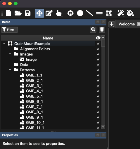
Fig. 4 A screenshot of the Items Panel in iolite Targeting
Clicking to expand a region will show sub-folders for the alignment points, images, data, and ablation patterns of that region. Clicking on any one of these subfolders will show the component images etc. Clicking on an item will show its properties in the Properties Panel, which is in the bottom left by default. The properties shown will depend on the pattern type. For example, clicking on an ablation pattern (e.g. spot, raster etc) will show the ablation properties of that pattern, including spot size, rep rate, fluence etc in the Properties Panel. Selecting an image will show information about the image in the Properties Panel, along with a control for setting the image opacity.
At the top of the Items Panel are the Filter, and buttons. The Filter button is used to filter the items shown in the Items Panel according to their attributes (e.g. spot size, metadata values etc). The button is used to zoom to the selected item(s) in the Main Panel. The button is used to delete the currently selected item(s).
Properties Panel
The Properties Panel displays properties of the currently selected item in the Items Panel.
When an ablation pattern(s) is selected in the Items Panel, the properties displayed will include the spot size, rep rate etc. More detail about ablation properties is included below.
When a region is selected, the region’s name and physical size are displayed.
When an image is selected, the properties shown will include the image source, physical size, and a slider control for adjusting the opacity of the image. Clicking the … button with an image selected will show the image in your systems default image viewer.
When an alignment point is selected, the name assigned to the alignment point, its x, y position and the size of the image captured along with the alignment point are displayed. When an alignment point is created, an image of the area surrounding the point is stored with the point (for ESL systems only). This is used for context when re-coordinating in AV2. The size of the image captured can be adjusted in the Properties Panel to provide additional context, at the expense of additional file size of the resulting LAX file.
Tip
Increasing the size of the image captured with an alignment point can provide more context during re-coordination.
The name of the selected object(s) is shown at the top left of the Properties Panel. This can be used to rename objects, perhaps most usefully for renaming ablation patterns. The button to the right of the name can be used to add a numbered suffix to the selected items.
Tip
To batch rename ablation patterns, select the patterns in the Items Panel and type the new name into the name field. Then, click the button to add a numbered suffix to each pattern (if required).
Setting ablation properties
If an ablation pattern is selected, the Properties Panel shows the ablation aperture size, rep. rate, fluence etc (Fig. 5). If multiple ablation patterns are selected, changes made in the Properties Panel apply to all selected patterns, and an icon representing layers will appear in the top right.
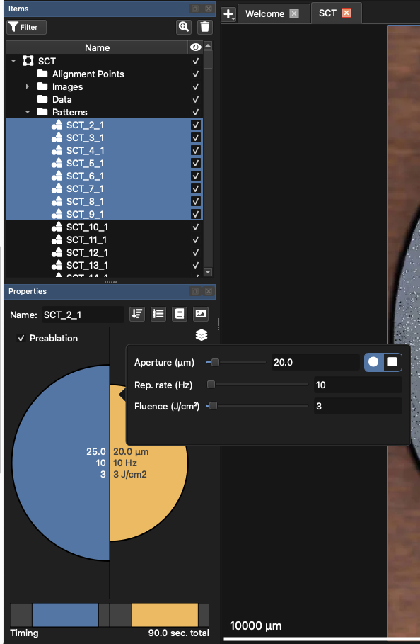
Fig. 5 A screenshot of the Properties Panel showing ablation properties for a selection of spot patterns
The button sorts the selected patterns by attribute. The button applies a suffix to selected patterns. For example, if the selected patterns are labelled “Samp_1”, “Samp_2”, “Samp_3” etc, clicking this button will add a suffix of “_1” to rename the patterns “Samp_1_1”, “Samp_2_1”, “Samp_3_1” etc. The button opens the Metadata window (described below). The button opens the Precognition Helper (described below).
Ablation properties can be adjusted by clicking the orange shape representing the laser spot (an orange circle in Fig. 5). This will show sliders controls and numeric fields for setting the apeture, rep. rate and fluence. To change the spot shape between circular and square, click the circle or square in the top right of this dialog.
If the pattern is a line, controls for setting the spot overlap will also be shown. Adjusting the overlap changes the scan speed, which is also visually represented as a dashed outline showing how far the ablation area will move between pulses. If the pattern is a raster or lasso pattern, controls for setting the line spacing will be shown in addition to the line properties previously described.
Checking the “Preablation” checkbox in the top left of the panel will add a preablation to the selection patterns, and the preablation properties will be shown in the left side of the panel. In the example in Fig. 5, the preablation spot size is 25 µm, and the main ablation spot size is 20 µm. The rep rate and fluence is 10 Hz and 3 J/cm², respectively, for both the preablation and main ablation.
At the bottom is the Timing Bar for the selected patterns. The colored portions (blue for preablation, if selected, and orange for main ablation) have a warmup time and washout time after each of them. Double clicking on the warmup, (pre)ablation, or washout intervals allows you to enter new timing values.
At the bottom, you’ll find the Timing Bar, which shows the duration for each part of the selected patterns. The grey area on the left represents the ‘Warmup’ time before the (pre)ablation. The colored section (e.g., blue for preablation, orange for main ablation) shows the duration of the ablation. The grey area on the right represents the ‘washout’ time after the ablation concludes.
You can change these times by double-clicking directly on any of these three sections (Warmup, (Pre)Ablation, or Washout) in the bar and entering a new value. For example, to change the warmup time of the main ablation to 5 seconds double click on the grey area before the main ablation event and change the value to 5 s.
Metadata Window
Metadata are data associated with patterns that are not related to the ablation itself. This might include data such as the sample name or ID, compositional information collected by a previously applied technique, or shape data determined during automatic grain finding.
When using ESL systems, the metadata will be added to the LAX file and when the LAX file is loaded into iolite v4, the metadata become properties of the selection. This allows the analyst to plot results calculated in iolite v4 against metadata values, such as grain area. Metadata fields, which are shown as columns in the Metadata window, can be added and removed using the and buttons in the top left of the window.
To set or adjust metadata for patterns, select the patterns in the Items Panel, and click the button at the top of the Properties Panel (top right). This will show the Metadata Window (Fig. 6).

Fig. 6 A screenshot of the Metadata window
Metadata are described in terms of a key (a name for each property, e.g. “area”) and a value. There is one key per property, and a value for each pattern, even if this value is blank. In Fig. 6 the keys are “area”, “circularity”, “convexity”, etc which are added automatically by the automated grain finding process. Custom metadata keys can also be created. Keys are shown as columns, and values are shown as cell entries in the Metadata Window.
To add a key, click the button. To remove a key, click the button. All values for that key will be deleted for the patterns selected, but if other patterns still have this key, their values will remain.
To edit any value, double-click on it in the table. To edit multiple entries, select the cells to be changed and click the button. Enter a value and click OK to set the value for all selected cells. To clear values for multiple entries, select the cells to clear and click the button.
The ‘From Items’ button collects metadata from items that overlap with the selected patterns. For example, spots placed on an image will have metadata fields added for the color intensities of the pixels at the spot’s center. Fields for the red, green and blue channels, as well as a calculated gray field will be added for the selected patterns.
Precognition
More details coming soon!
Review Mode
Review Mode is a quick way to view patterns within a Region to check and adjust their placement and potentially delete any that are not needed or incorrectly placed. To enter Review Mode, click the button in the toolbar (top right corner of the main window).
When Review Mode is entered a small panel on the bottom right of the main window will appear showing the controls for moving between patterns
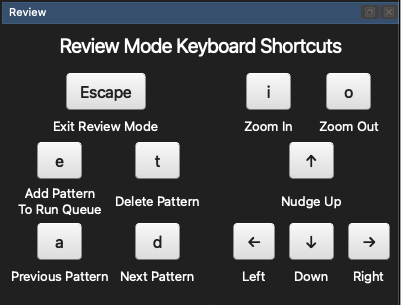
Fig. 7 The Review Mode panel that is shown when Review Mode is active.
When in Review Mode, you cannot change or close region tabs. You must exit Review Mode before changing region.
To move between patterns, use the a (previous) or t (next) keys on the keyboard, or press the buttons in the Review Mode panel.
To adjust a pattern’s position, you can nudge the pattern up, down, left or right using the arrow keys on the keyboard, or press the buttons in the Review Mode panel.
To delete a pattern, press the t key. To add a pattern to the run queue, press the e key (or alternatively, after finishing your review add all patterns at once by dragging them to the Run Order List).
To zoom in or out while in Review Mode, press the i (zoom in) or o (zoom out) keys.
To exit review mode, please the escape key or press the Escape button in the Review Mode panel. You can also exit Review Mode by clicking the button again in the toolbar (it will no longer be highlighted when Review Mode is not active).