Automated Mineralogy and iolite Targeting
Combining automated mineralogy with LA-ICP-MS has many benefits, including providing independent major element concentrations to use as internal standards for LA-ICP-MS data processing, as well as creating rich datasets with major, trace and ultra-trace element information. iolite Targeting streamlines the process of connecting automated mineralogy (SEM) results with LA-ICP-MS patterns and results in iolite v4 and reduces the chances of user errors when combining SEM and LA-ICP-MS datasets.
iolite Targeting supports automated mineral datasets from the following instruments:
The following guide presents a simple workflow for each of these instruments. It assumes a basic knowledge of Targeting, for example, having worked through the two examples in the Guided Introduction. If you are a beginner to iolite Targeting there are full instructions and example datasets to get you started there.
TIMA
There are two main ways to interact with TIMA data in Targeting. The first is importing a panorama image and grain list Excel spreadsheet. This approach has the advantage that it can propagate individual grain concentration data through the LA-ICP-MS process. The disadvantage is that it is a two step import process, only includes the grains included in the Excel spreadsheet exported from the TIMA software, and that no scale information is recorded with the image and so must be entered by the user.
The other approach is to import the MINDef database exported from the TIMA software. This has the advantage that back-scattered electron (BSE) images are imported, all phases are present and automatically selectable, and scale information is stored with the database. However, it does not include grain-by-grain concentration data.
A guide to both approaches is provided below.
Panorama and Excel Import
Panorama images can be imported using the + button like other images. However, unlike most images, the coordinate system for the panorama image must be set to ensure that the coordinates recorded in the Excel grain list align correctly with the image.
If your panorama image includes a title bar at the top or an information panel at the bottom (e.g., scale bar, phase‑colour legend), we recommend creating a copy of the file and cropping these elements off. Doing so ensures that the image centre corresponds to the (0, 0) coordinate.
Alternatively, you may calculate how many pixels the title bar and information panel add to the image and then determine the true centre coordinate. This approach is more complex, which is why cropping is generally preferred. If you do remove the scale bar during cropping, make sure to record the exact width or height of the resulting image, as you will need to enter this information in the next step.
Click the + button and select “Image” from the list of options. Select your image file and click OK. Select the “Centre” option in the bottom left of the Image Import window, and set the starting coordinates (0, 0 if you have cropped your image as described above). Select which dimension you want to enter to determine the image scaling using the control at the top centre of the Image Import window (either “Width” or “Height”). Click OK and give your Region a name. Click OK and enter the scaling information (width or height). Click OK and your image is now set up within your new region.
At this point, you could manually add points, lines, rasters etc like any other image. However, we are going to use the information in the Excel grain list file to automatically create targets.
The Excel file must contain the x and y coordinates as columns in addition to any other data you wish to import, such as grain ID, grain area, dataset name, and any compositional data for each grain.
To import the Excel file, click the + button and select “Data”. Select the grain viewer Excel file and click OK. This will show the Data Import window. At the top of the window, change the import type from “Region” to “Data In Region”. This will add the data to the existing region instead of creating a new region.
There are two tabs in the Data Import window: Data and View. The Data tab shows a preview of the data to be loaded along with some controls at the bottom for adjusting how many header and footer rows the file contains etc. The View tab shows how the data would be distributed given the x and y information provided (it may show nothing to start with).
Start in the Data tab. If this is the first time loading a grain viewer Excel file, the “Header Rows To Ignore” and “Footer Rows to Ignore” may already be set to 0, and the “My file has a header row” option may be unchecked. The column titles will likely show numbers instead of their proper names.
Start by selecting the “My file has a header row” option. The column titles will now likely show “Grain view” and “Unnamed: 1”, “Unnamed: 2”, etc. Increase the “Header Rows To Ignore” value until the column titles match the names in the file (e.g. Grain, X[µm], Y[µm], etc). Scroll to the bottom of the table to check that there are no footer rows (i.e. rows that do not match the main data format). If there are none, the “Footer Rows To Ignore” can be left at 0.
In the View tab, select the column names for the columns containing the x and y values. This will likely be something like X[µm] and Y[µm]. Select the “Use raw coordinates” and “Flip y coordinates” options. Click OK to finish the data import. In your region, you should now be able to see each of the datapoints (each row in the spreadsheet) in the Data folder of the region. Select a datapoint and right click on it, and select “Show data” to see the metadata imported with that point in the Data Viewer window. Close the Data Viewer window to continue.
By default each datapoint will be plotted in the main viewing area as a small blue circle. You can adjust the size and color of this circle using the size field (which by default is size 50) and the color picker button (a colored button with … on it). Depending on the color of the phases in your panorama, you may need to adjust the color for the points to be visible.
Note
The following explanation of filtering datapoints is optional and filtering can be applied when creating ablation patterns. However, filtering of data points may help you explore your data and aid in targeting strategy.
Now the datapoints can be filtered using the Filter button at the top of the Items Panel. Click the Filter button to show the filters sub-panel. Click the + button in this filters sub-panel to add a new filter. A new filter will be added to the table of filters, and will have a small warning symbol indicating that the filter is not correctly set yet. Double-click in the Attribute field to add a value to filter by. Datapoint metadata fields can be entered by typing “data.” and a list of metadata fields will appear (e.g. “data.Area[px]”). Select the value you want to filter by. Double click on the comparator value to change between “equal to”, “greater than”, etc. Then enter the filter value. If the filter is valid, the warning symbol will disappear. Only points matching the filter will be shown. Additional filters can be added using the + button. Filters can be combined so that points matching any filter will be shown using the “Any” button in the top right of the filter sub-panel. Otherwise, datapoints must match all filters to be shown. Filtering of datapoints is also discussed here.
An alternative approach to filtering datapoints in this way is to create a copy of your Excel file, and filter the datapoints in Excel before importing the file into Targeting.
Patterns can be created from each datapoint in two ways: a simple spot pattern applied as each selected datapoint, or more advanced patterns that may require determining each grain’s boundaries using a flood fill algorithm.
Select the datapoints to create patterns for in the Items Panel. In the Properties Panel below the Items Panel, click the “Create Patterns” button. A window will appear asking if you want to create simple spot patterns (one spot pattern centered on each datapoint) or “Advanced Patterns”. This guide will show the Advanced Patterns option as the simple spot patterns approach is relatively self-explanatory. Select “Advanced Patterns” and click “OK”.
A window will appear with options for the pattern type and placement strategy. In this example we’ll use a lasso example. Select Lasso from the pattern type options. For the settings, choose your spot size. The “Buffer” variable determines how far out from the grain edge to extend the lasso. This is normally to ensure that some of the background is included in the lasso. For example, a value of 5 for the buffer will expand the lasso 5 µm outside the grain’s boundary. Leave it as 0 to cover only the grain area.
The Epsilon value is a shape simplification factor. Simplifying the grain outline can avoid adding extra scanlines just for small protuberances on the edge of the grain, although excessive epsilon values will oversimplify the grain boundary and may miss areas. a value between 1 and 2 for epsilon is typically satisfactory. A description of filters is included here.
Click OK to create a lasso pattern for each grain selected. A window will appear asking for a base-name for each pattern. For example, choosing “spot” as the base-name will create patterns with labels like “spot_1”, “spot_2”, etc. Click OK to finish creating patterns from the datapoints.
To copy the metadata from the datapoints to the patterns, select the patterns in the Items Panel, and click the (metadata) button in the Properties Panel. This will show the metadata for each selected pattern. Click the From Items button to automatically copy metadata from the datapoints to the patterns. This will include any compositional information that can later be used by iolite v4 for internal standard corrections etc.
At this point, the experiment is ready for adding alignment points and setting up the run order list, as described in the guided guided examples.
MINDef Database Import
The MINDef database should be part of a folder structure that contains the database (typically called “data.sqlite”) and a sub-folder with the name of the experiment ID (usually a long string of letters and numbers). Within this subfolder, there should be three .xml files:
fields.xml
measurement.xml, and
phases.xml
There should also be a folder called “fields”. This fields sub-folder contains each field’s BSE, mask and phases image.
Click the + button and select “Tescan TIMA”. Select the folder containing the database file and the subfolder with the experiment ID and click OK. It will take a few seconds to read the database and open and place each field’s BSE image into a combined image. A preview of the image will be shown in the TIMA Fields and Database Import window. Click OK to continue. A window will appear asking for a label for the region. Add the region’s name and click OK.
A new region will be created for the sample. It will initially have just a single item: the combined BSE image containing all the fields stitched together.
Tip
If the contrast of the combined BSE image is too low, you can use iolite Targeting’s builtin tools to adjust the contrast. Just note however that the original image must be selected to follow the rest of this guide.
Select the combined BSE image in the Items Panel. In the Properties Panel below a menu labelled “Class” will appear showing the names of the phases present in the sample, listed in descending order of abundance. Selecting the phases name will highlight that phase in the main viewing area (if you have any other images in the region, make sure they are not visible or are beneath the original BSE image for the highlighting to be visible). Phases will be colored according to the color scheme stored in the phases.xml file, which is exported from the TIMA software.
To create patterns for a phase, click the |shapes| Create Patterns button. A window will appear with options for the targeted material, the pattern base-name, and filters for filtering which grains to target. Select the material to be targeted at the top of this window, provide a base-name for the patterns (e.g. “epidote” as the base-name will create patterns with labels like “epidote_1”, “epidote_2”, etc), and add any filters for area, circularity, convexity etc as needed. Checking the checkbox in the Enabled column enables the filter. A description of filters is included here.
Tip
Due to grains being listed multiple times in the database, it is recommended that you enable the “Distance” filter. Any grains within this value (in µm) of a target grain will be ignore. This avoids multiple patterns for the same grain. A reasonable starting point for the value to use could be half the minimum grain area filter.
Choose the pattern type at the bottom of this window (Spot, Line, Raster or Lasso), and the strategy type. Click the button to set the buffer and epsilon values, as well as the spot size. Click the Target button to create the patterns.
The patterns should now appear in the region. This process can be repeated for all classes and pattern types needed. At this point, the experiment is ready for adding alignment points and setting up the run order list, as described in the guided guided examples.
Brüker AMICS
iolite Targeting can natively read AMICS .bin files. To import an AMICS file click the + button and select “Bruker AMICS”. Select the .bin file from the AMICS software and click Open. A preview of the file will be shown. Click the OK button to finish the import. A new region will be created with the backscattered electron image as the only item in the region’s images folder.
Clicking on the image will show a “Class” menu and “|shapes| Create patterns” button in the Properties Panel. Selecting a mineral/phase name in the Class menu will highlight that class in the main viewing area. Normal spots, lines, rasters or lasso patterns can be placed manually at this point.
Ablation patterns can then be added as described below.
Thermo Maps Min
iolite Targeting can read the database and image files created by Thermo Fisher’s Maps Min software. To import a Maps Min dataset, click the + button and select “Thermo Maps Min”. You will be prompted to select the XrayData.db file for your dataset. Targeting assumes that there will be two folders in the same directory as the XrayData.db file: a folder called “BSE” and another called “classification-results”. Both of the latter folders contain images of the sample. Select the .db file and click Open. The SEM Import window will appear.
At the top of the window, there is a dropdown menu for selecting which image to preview in the window. There is also a menu to select which phase maps and concentration images to import into Targeting. There are “Select All” and “Select None” controls at the end of the list to help with selecting the images. Typically the BSE and any composition images that you would like to associate with your LA-ICP-MS results would be imported. Targeting will store the selection of images imported so that next time you import a file of this type, the images will be automatically selected. Click the OK button to finish the import.
Once the dataset is imported, you can right-click on any image in the list of images and select “Raise to top” to make it the visible image. Alternatively, you can select the image you want to see and press Ctrl+t (Cmd+t on Mac) to toggle off all images except the currently selected image. By default, most SEM images are initially shown with a grey-scale gradient. To change the color gradient, click on the image shown and in the Properties Panel, select a colormap from the Colormap downdown menu.
Tip
Colormaps with names ending in “S” are for categorical data c.f. to typical colormaps that are gradational between values. Using a categorical colormap helps highlight the differences between phases.
To highlight the automated mineralogy phases over an image, click on the image in the list, and in the Properties Panel, select the phase from the Class dropdown menu. By default, this will highlight the grains of the class using the colors from Maps Min. Click the button beside the class dropdown menu to adjust the highlight color.
Note
Phase maps do not need to be imported along with the composition images. Targeting will use the database file to determine the location of grains of different phases.
Ablation patterns can then be added as described below.
Zeiss Phase Identifier AI
iolite Targeting can read .czi file exported from the Zeiss Phase Identifier AI software. To import a CZI file click the + button and select “Zeiss CZI”. Select the .czi file and click Open. A preview of the file will be shown, displaying the segmented phase map. The image shown in the preview can be changed by selecting a different image the Preview menu in the top top. An image for each chemical map in the CZI file is available for preview. As no scaling information is included in the CZI file (at the time of writing) the scaling information needs to be manually set. Select a dimension to enter the details for with the Scale menu at the top of the window (either “Width” or “Height”). Click the OK button to finish the import. You will be prompted for a name for the sample and the scaling information. A new region will be created with all the images in the CZI file available as images.
Tip
The order of the images in the Images folder represents their z ordering. That is, the first image in the list is the top-most image, and the last image in the list is at the bottom. You can move an image up, down, to the top, or to the bottom by right clicking on it and selecting the appropriate item.
Tip
To make the currently selected image visible and all other images non-visible, use the keyboard shortcut Ctrl+t (Cmd + t on Mac).
Images are automatically min-max scaled to reveal features in the images, but additional contrast adjustment can be applied using Targeting’s image adjustment tools.
Selecting any image from the CZI file in the Items Panel will show a Class menu and “|shapes| Create Patterns” button in the Properties Panel. Selecting a mineral name from the Class menu will highlight the class in the main viewing area. Ablation patterns can be manually added at this point, following the instructions below.
Creating Patterns from AM grains
To automatically place patterns on grains, click the “|shapes| Create Patterns” button. A window will appear with options for the Material/Class to target, the pattern base-name, and filters to be applied (Fig. 31). A description of filters is included here. The pattern type, along with targeting strategies (discussed here), can be set at the bottom of the window. The minimum distance filter will remove any targets within the given distance (in µm) of an existing pattern. The order in which patterns are added affects this filter.
There is an option labelled “Capture metadata to be stored with generated patterns?”. Checking this option will calculate the mean value of each of the imported images within the area defined by each the ablation pattern. For example, if the Fe, O and Si images have been imported (or the data are available via the binary file or database file), for each ablation pattern, the average of the Fe pixels within a polygon that defines that pattern will be stored as metadata with that pattern. This allows storing of major element information for each pattern that can be used for internal standard calculations in iolite v4. Checking this option will increase the amount of time taken to generate each of the patterns while the average is determined and stored as metadata, but this additional time is usually less than a few seconds.
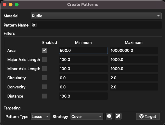
Fig. 31 Options for creating patterns from SEM classes
Once the pattern type and strategy has been chosen, and the strategy options selected in the menu, click the Target button to create the patterns. If the option to capture metadata was selected, each pattern will now have the associated results stored as metadata, which is viewable in the Metadata Window. Morphology data such as circularity and grain area will also be stored as metadata for use in iolite.